디지털 신호처리 프로젝트 - FIR, IIR 필터 설계

소개글

디지털 신호처리 프로젝트 - FIR, IIR 필터 설계에 대한 보고서 자료입니다.

목차

1. Excutive Summary
* 과제의 목적
* Problem Statement
* Approach
* 결과 및 결론

2. 본론

3. MATLAB Source Code

본문내용

tude\')
figure(4),subplot(5,1,4),plot(f,fftshift(Wo4))
title(\'signal at freq domain filtering by window4\'),xlabel(\'freq\'),ylabel(\'amplitude\')
figure(4),subplot(5,1,5),plot(t,a4,\'r\',t,ot4,\'g\')
title(\'signal at time domain filtering by window4\'),xlabel(\'time\'),ylabel(\'amplitude\')
Project3 - (1)의 소스코드
A=1;B=1;C=1;D=1; %arbitary mixing parameter
AP=0;BP=0;CP=0;DP=0; % arbitary phase component
t0 = 1;
ts = 0.001;
fs = 1/ts;
t = [0:ts:t0];
f = [-0.5*(1/ts):1/t0:0.5*(1/ts)];
a1=A*cos(2*pi*50*t+AP);
a2=B*cos(2*pi*70*t+BP);
a3=C*cos(2*pi*100*t+CP);
a4=D*cos(2*pi*120*t+DP);
ot=a1+a2+a3+a4; % original 신호
Of=fft(ot)/fs; % original 신호의 주파수 영역 표현
%%%%%%%%%%%%%%%%%%%%%%% awgn 잡음 추가 신호 %%%%%%%%%%%%%%%%%%%%%%%%%%%%%
S = power(ot(1:length(t)),2); %ot의 전력
N = S/20; %20dB (SNRdB)
N_std = sqrt(N); %평균이 0인 잡음의 전력= 분산을 통해 표준 편차를 구함
Nt = N_std.*cos(2*pi*250*t); %표준편차 N_std인 250Hz cosine 잡음
ot_awgn = ot + Nt; %잡음이 섞인 신호
Of_awgn=fft(ot_awgn)/fs;
subplot(4,1,1),grid,plot(t,ot),axis([0, 0.1, -10, 10])
title(\'time domain - original signal\')
subplot(4,1,2),grid,plot(t,ot_awgn),axis([0, 0.1, -10, 10])
title(\'time domain - original signal + 250kHz frequency noise \')
subplot(4,1,3),plot(f,abs(fftshift(Of))),axis([-500, 500, 0, 0.6])
title(\'freq. domain - original signal\')
subplot(4,1,4),plot(f,abs(fftshift(Of_awgn))),axis([-500, 500, 0, 0.6])
title(\'freq. domain - original signal + 250kHz frequency noise\')
Project3 - (2) ,(3)의 소스코드
A=1;B=1;C=1;D=1; %arbitary mixing parameter
AP=0;BP=0;CP=0;DP=0; % arbitary phase component
t0 = 1;
ts = 0.001;
fs = 1/ts;
t = [0:ts:t0];
f = [-0.5*(1/ts):1/t0:0.5*(1/ts)];
a1=A*cos(2*pi*50*t+AP);
a2=B*cos(2*pi*70*t+BP);
a3=C*cos(2*pi*100*t+CP);
a4=D*cos(2*pi*120*t+DP);
ot=a1+a2+a3+a4; % original 신호
Of=fft(ot)/fs; % original 신호의 주파수 영역 표현
%%%%%%%%%%%%%%%%%%%%%%% awgn 잡음 추가 신호 %%%%%%%%%%%%%%%%%%%%%%%%%%%%%
S = power(ot(1:length(t)),2); % ot의 전력
N = S/20; %20dB (SNRdB).
N_std = sqrt(N); % 평균이 0인 잡음의 전력= 분산을 통해 표준 편차를 구함
Nt = N_std.*cos(2*pi*250*t); % 표준편차 N_std로 퍼져있는 250Hz cosine 잡음
corrupted = ot + Nt; % 잡음이 섞인 신호
W1=[ones(1,150),zeros(1,700), ones(1,151)]; % +-150Hz 사이 통과 필터 (저역통과필터 기능)
Corrupted=fft(corrupted)/fs; % 잡음 추가신호의 주파수영역 표현
Wo=Corrupted.*W1; % 잡음제거신호, 즉, finally신호의 주파수 영역 표현
finally=ifft(Wo).*fs; % finally신호의 역 푸리에 변환 => 시간영역 표현
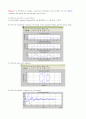
subplot(6,1,1),plot(f,abs(fftshift(Corrupted)))
title(\'corrupted - freq. domain\'),xlabel(\'freq\'),ylabel(\'amplitude\')
subplot(6,1,2),plot(f,fftshift(W1));
title(\'window - filter\'),xlabel(\'freq\'),ylabel(\'amplitude\')
subplot(6,1,3),plot(f,fftshift(Wo)),axis([-500,500,0,1]);
title(\'finally filtering by corrupted - freq.domain \'),xlabel(\'freq\'),ylabel(\'amplitude\')
subplot(6,1,4),plot(t,ot)
title(\'original signal - time domain.\'),xlabel(\'time\'),ylabel(\'amplitude\')
subplot(6,1,5),plot(t,finally,\'g\',t,ot,\'r\')
title(\'finally versus original signal - time domain\')
subplot(6,1,6),plot(t,corrupted,\'r\',t,ot,\'g\')
title(\'corrupted versus original signal - time domain\'),xlabel(\'time\'),ylabel(\'amplitude\')
Project3 - (6) ,(7)의 소스코드

키워드

성균관대,   디지털신호처리 ,   DSP,   DSP 프로젝트,   FIR,   IIR,   필터,   필터 설계